Azure Managed Redis: vector search, HNSW, FLAT, Hash, and JSON

radio_button_uncheckedshort_text1. The semantic retrieval problem and learning goals

An enterprise knowledge assistant may hold millions of technical documents while users expect a relevant answer in milliseconds. Keyword matching alone cannot capture intent reliably, so the application converts documents and questions into high-dimensional embeddings. Similar concepts occupy nearby positions, which makes distance a practical signal for semantic retrieval, recommendations, Retrieval-Augmented Generation (RAG), and related AI workloads.

A production design must do more than compare vectors. It must preserve the embedding dimension and numeric type, store searchable metadata, choose exact or approximate indexing, update records, filter by authorization or department, and measure the balance among latency, recall, memory, and cost. This chapter uses a 1,536-dimensional document model as a running example without assuming that every model has that size.

• Create RediSearch vector schemas and ingest embeddings with redis-py.
• Run KNN, range, and hybrid metadata-filtered queries.
• Choose FLOAT32 or FLOAT64, a distance metric, and FLAT or HNSW from measured workload requirements.
• Select Redis Hash or Redis JSON and plan safe migrations and reindexing.
• Build and validate a Python semantic-search application on Azure Managed Redis.

Topic summary

Vector retrieval is a complete data-and-query design problem: model output, schema, metadata, index, runtime parameters, and operational measurements must agree.

radio_button_uncheckedshort_text2. Provision Azure Managed Redis for vector search

Azure Managed Redis exposes vector capabilities through the managed RediSearch module. Enable RediSearch when the instance is created because modules cannot be added later. The current service also requires the Enterprise clustering policy, the NoEviction policy, and a supported in-memory tier: Memory Optimized, Balanced, or Compute Optimized. Flash Optimized does not support RediSearch.

Size both the stored records and the secondary-index overhead. Use TLS for client connections; prefer Microsoft Entra ID authentication where the client supports it; and evaluate Private Link, high availability, diagnostics, and recovery requirements for production. Azure manages module versions, so the application should test behavior against the service version rather than assuming a manually installed Redis module.

Topic summary

Vector search begins at provisioning: RediSearch, Enterprise clustering, NoEviction, a compatible tier, and sufficient index memory must be selected up front.

radio_button_uncheckedshort_text3. From content to indexed results

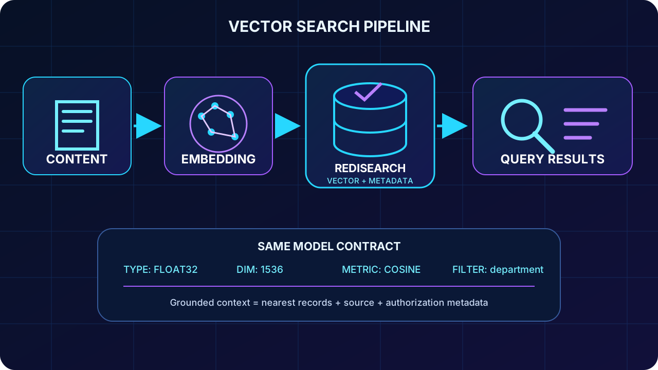
The application first divides source content into retrievable units, obtains one embedding per unit, and writes the vector together with identity, source, category, timestamp, tenant, and access-control metadata. RediSearch watches keys that match the index prefix and updates its secondary index. A question follows the same embedding model and preprocessing path, then KNN or range search compares the query vector with indexed vectors.

Metadata serves two purposes: it narrows candidates before vector comparison and gives the final answer traceable sources. In RAG, the application retrieves the original text and provenance from the selected records, constructs grounded context, and sends that context to the generation model. Vector distance ranks candidates; it does not by itself authorize access or prove factual correctness.

Topic summary

Index documents and query text with the same embedding contract, keep provenance and access metadata beside each vector, and treat retrieval as ranking rather than authorization.

radio_button_uncheckedshort_text4. Define a vector index over Redis Hash

A RediSearch schema describes fields that can be searched or returned. The vector field declares an algorithm, numeric TYPE, DIM, and DISTANCE_METRIC. Text and tag fields make hybrid filtering possible. An IndexDefinition limits indexing to a key prefix and specifies whether the source documents are Hash or JSON.

from redis.commands.search.field import TagField, TextField, VectorField
from redis.commands.search.indexDefinition import IndexDefinition, IndexType

schema = (
    TextField("title"),
    TagField("department"),
    VectorField("embedding", "HNSW", {
        "TYPE": "FLOAT32",
        "DIM": 1536,
        "DISTANCE_METRIC": "COSINE",
        "M": 16,
        "EF_CONSTRUCTION": 200,
    }),
)

client.ft("idx:documents").create_index(
    schema,
    definition=IndexDefinition(
        prefix=["doc:"],
        index_type=IndexType.HASH,
    ),
)

The example uses HNSW, FLOAT32, 1,536 dimensions, and cosine distance. M and EF_CONSTRUCTION influence graph connectivity, memory, build time, and recall; they are construction-time settings, not cosmetic values. The prefix doc: prevents unrelated keys from entering the index. Schema creation should be an explicit deployment step with versioning and rollback, not an implicit action on every application startup.

Topic summary

A vector index must bind algorithm, type, dimension, metric, searchable metadata, source data type, and key prefix into one stable schema.

radio_button_uncheckedshort_text5. Store vectors and metadata correctly

Hash vector fields use compact binary blobs. Convert the model output to the exact NumPy dtype declared in the index and verify its one-dimensional shape before calling tobytes(). Human-readable fields remain normal Hash values. A 1,536-value FLOAT32 embedding occupies 6,144 bytes before Redis object, metadata, replication, and index overhead.

import numpy as np

embedding = np.asarray(model_embedding, dtype=np.float32)
if embedding.shape != (1536,):
    raise ValueError("The embedding must contain exactly 1536 values")

client.hset("doc:917", mapping={
    "title": "Model deployment runbook",
    "department": "engineering",
    "content": "Operational steps for model deployment...",
    "embedding": embedding.tobytes(),
})

Dimension mismatches and dtype mismatches can fail indexing or make queries invalid. Do not silently truncate, pad, or reinterpret vectors. Store the embedding model and version in metadata when more than one generation can coexist; a model migration normally needs a separate field or index until all vectors and query clients use the new contract.

Topic summary

For Hash, serialize the exact indexed dtype to bytes, validate DIM, retain useful metadata, and version the embedding contract.

radio_button_uncheckedshort_text6. Batch ingestion, updates, and indexing visibility

One network round trip per document becomes expensive during a large load. A redis-py pipeline batches commands and sends them together. transaction=False makes the intent explicit: this is throughput batching, not one all-or-nothing transaction. Choose bounded batches to avoid excessive client memory, server queues, or long retries.

with client.pipeline(transaction=False) as pipe:
    for document in documents:
        vector = np.asarray(document["embedding"], dtype=np.float32)
        pipe.hset(f'doc:{document["id"]}', mapping={
            "title": document["title"],
            "department": document["department"],
            "content": document["content"],
            "embedding": vector.tobytes(),
        })
    responses = pipe.execute()

# Batching reduces network round trips; it does not make the whole load atomic.
assert all(result >= 0 for result in responses)

RediSearch maintains the index as matching keys change. After a bulk load, verify document counts and run representative queries before declaring the dataset ready. For retries, use deterministic keys so repeated writes replace the intended record. Record failures from execute(), apply backoff, and make model/version transitions observable. Pipeline speedups depend on network, payload, and server load; benchmark instead of promising a fixed multiplier.

Topic summary

Pipelines reduce round trips, deterministic keys make retries safe, and post-load count and query checks prove that indexing is usable.

radio_button_uncheckedshort_text7. Run a K-nearest-neighbor query

KNN asks for a fixed number of nearest records. The query syntax names K, the vector field, the binary parameter, and a distance alias. Return only fields needed by the application and sort by distance. Redis vector queries use dialect 2; recent redis-py versions request it by default, but declaring it keeps the example portable and readable.

from redis.commands.search.query import Query

query_vector = np.asarray(query_embedding, dtype=np.float32).tobytes()
query = (
    Query("*=>[KNN 5 @embedding $query_vec AS vector_distance]")
    .return_fields("title", "department", "vector_distance")
    .sort_by("vector_distance")
    .dialect(2)
)

results = client.ft("idx:documents").search(
    query,
    query_params={"query_vec": query_vector},
)

With COSINE, lower distance means closer vectors: zero represents identical direction and values can approach two for opposite directions. The score is not a universal probability or confidence value. Calibrate acceptable distances on labeled examples from the actual model, language, content domain, and chunking strategy.

Topic summary

KNN returns the closest K records; bind the query vector as bytes, sort by the distance alias, and interpret distance only within a calibrated workload.

radio_button_uncheckedshort_text8. Combine semantic similarity with metadata filters

Hybrid search restricts candidates using indexed metadata and then ranks them by vector distance. A support assistant can limit results to one product, a knowledge portal to the engineering department, and a multi-tenant system to the current tenant and permitted classifications. Filtering is therefore part of correctness and security design, not merely an optimization.

query = (
    Query(
        "@department:{engineering}=>"
        "[KNN 3 @embedding $query_vec AS vector_distance]"
    )
    .return_fields("title", "department", "vector_distance")
    .sort_by("vector_distance")
    .dialect(2)
)

Tag values that contain reserved query characters must be escaped or modeled safely. Apply every mandatory authorization predicate server-side and still validate returned records in the application. Measure selectivity: restrictive filters may accelerate comparison, while an unsuitable index or skewed field can produce unexpected latency.

Topic summary

Hybrid queries combine mandatory metadata constraints with vector ranking; filters must be indexed, escaped correctly, and enforced as part of the authorization boundary.

radio_button_uncheckedshort_text9. Use vector-range queries for thresholds

KNN always targets a fixed result count, even when the nearest candidates are poor. VECTOR_RANGE instead returns records within a maximum distance, so the result count can be zero or many. This is useful for semantic caches, duplicate detection, and retrieval flows that should decline to answer when no source is sufficiently close.

query = (
    Query(
        "@embedding:[VECTOR_RANGE $radius $query_vec]"
        "=>{$YIELD_DISTANCE_AS: vector_distance}"
    )
    .return_fields("title", "vector_distance")
    .sort_by("vector_distance")
    .dialect(2)
)

results = client.ft("idx:documents").search(
    query,
    query_params={"radius": 0.20, "query_vec": query_vector},
)

Choose the radius from evaluation data, not intuition. The same numeric threshold has different meaning under COSINE, L2, or IP and under different embedding models. HNSW range search also supports EPSILON, which broadens candidate exploration and may improve recall at the cost of runtime.

Topic summary

Use KNN when the application needs K ranked candidates and VECTOR_RANGE when it needs every candidate inside a calibrated distance boundary.

radio_button_uncheckedshort_text10. Match numeric type and dimensions

Most embedding models are designed for FLOAT32, which usually halves vector payload memory relative to FLOAT64 and reduces transfer and computation costs. Current Redis versions can expose additional quantized types, but Azure Managed Redis controls the available module version; verify service compatibility and measured recall before choosing them. The source learning module focuses on FLOAT32 and FLOAT64.

DIM is fixed by the embedding model: 384, 768, 1,024, 1,536, and 3,072 are common examples, not interchangeable presets. Index, stored record, and query must have exactly the same element count and type. Changing models requires a planned re-embedding and reindexing process.

Topic summary

FLOAT32 is the normal AI default, while DIM and dtype must exactly match the model, stored bytes, index schema, and every query.

radio_button_uncheckedshort_text11. Choose COSINE, L2, or inner product

The correct metric comes from the embedding model contract and evaluation results. A mathematically valid metric can still rank semantic content poorly if the model was trained for another comparison. Normalize vectors only when the model and chosen metric require it; do not alter model output reflexively.

Topic summary

Select the distance metric the embedding model expects, then validate retrieval quality on representative labeled queries.

radio_button_uncheckedshort_text12. FLAT exact search versus HNSW approximate search

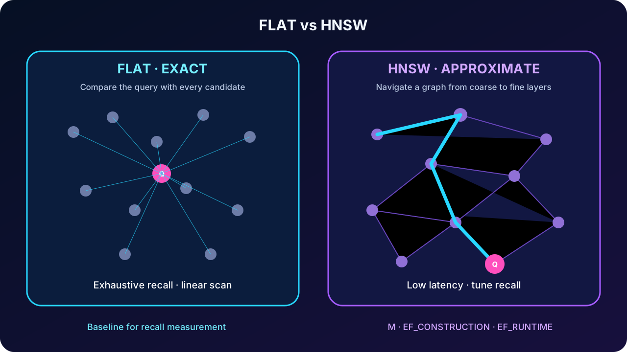
FLAT compares the query against every indexed vector and therefore provides exhaustive nearest-neighbor search. It is simple and exact but grows linearly with the candidate set. HNSW builds a multilayer navigable graph and visits a subset of promising nodes. It normally offers much lower latency at scale while accepting that an approximate search can miss a true neighbor.

Thresholds such as ten thousand or one million records are heuristics, not platform guarantees. Vector dimension, hardware tier, filter selectivity, concurrency, recall target, and memory budget can move the crossover substantially. Use FLAT as a ground-truth baseline when evaluating HNSW recall.

Topic summary

FLAT is exhaustive and predictable; HNSW trades some recall for scalable latency. Select with benchmarks rather than a fixed record-count rule.

radio_button_uncheckedshort_text13. Tune and benchmark HNSW

HNSW exposes construction and query controls. M increases graph connections, usually improving navigability while consuming more memory. EF_CONSTRUCTION widens neighbor exploration while building the graph, increasing build time and often recall. EF_RUNTIME controls the candidate set explored for each KNN query: raising it commonly improves recall but also raises latency. Defaults are starting points, not targets.

query = Query(
    "*=>[KNN 10 @embedding $query_vec EF_RUNTIME $ef AS vector_distance]"
).sort_by("vector_distance").dialect(2)

for ef_runtime in (10, 50, 100, 200):
    started = time.perf_counter()
    result = client.ft("idx:documents").search(
        query,
        query_params={
            "query_vec": query_vector,
            "ef": ef_runtime,
        },
    )
    latency_ms = (time.perf_counter() - started) * 1000
    evaluate(ef_runtime, latency_ms, result.docs)

Build a labeled query set and record p50, p95, and p99 latency, throughput, memory, index-build duration, and recall@K against FLAT results. Test production-like concurrency and metadata filters. Select the lowest-cost configuration that satisfies the agreed service objective and quality threshold; repeat after model, dataset, tier, or traffic changes.

Topic summary

Tune M and EF_CONSTRUCTION at index build time and EF_RUNTIME per query; compare HNSW recall with FLAT while measuring tail latency, throughput, and memory.

radio_button_uncheckedshort_text14. Model vectors in Hash or Redis JSON

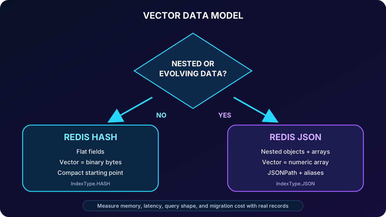
Hash stores a flat field-value record and represents the vector as compact binary bytes. It is a strong default when the schema is simple and memory efficiency and direct field operations matter. Redis JSON keeps nested objects and arrays naturally; vectors are stored as numeric arrays, while the binary query vector is still passed as bytes. JSONPath fields use aliases in the search schema to keep queries concise.

from redis.commands.json.path import Path

document = {
    "name": "Wireless headset",
    "price": 99.90,
    "category": "electronics",
    "specs": {"color": "black", "wireless": True},
    "embedding": embedding.tolist(),
}
client.json().set("jdoc:12345", Path.root_path(), document)

schema = (
    TextField("$.name", as_name="name"),
    TagField("$.category", as_name="category"),
    VectorField("$.embedding", "HNSW", {
        "TYPE": "FLOAT32", "DIM": 1536,
        "DISTANCE_METRIC": "COSINE",
    }, as_name="embedding"),
)

Topic summary

Choose Hash for compact flat records and JSON for nested or evolving documents; the source type, vector representation, and index definition must agree.

radio_button_uncheckedshort_text15. Migrate data structures and index versions safely

Changing Hash records into JSON changes the Redis key type and index definition. A safe migration writes converted documents under a new prefix, builds a new JSON index, validates counts and queries, switches readers deliberately, and retains the old dataset through a rollback window. Overwriting an existing Hash key with JSON is not a migration plan.

# Write transformed documents under a new prefix; do not overwrite Hash keys.
for key in client.scan_iter(match="product:*"):
    source = client.hgetall(key)
    vector = np.frombuffer(source[b"embedding"], dtype=np.float32)
    target = {
        "name": source[b"name"].decode(),
        "price": float(source[b"price"]),
        "category": source[b"category"].decode(),
        "embedding": vector.tolist(),
    }
    client.json().set(f"j{key.decode()}", Path.root_path(), target)

# Build and validate the JSON index, then switch reads deliberately.
# Keep the old index until validation and rollback windows are complete.

The same blue-green approach supports a model or dimension change: write a new embedding field or prefix, build a versioned index, backfill, compare retrieval, cut over, and only then remove the old version. Monitor indexing failures, memory pressure, rejected writes, query latency, and recall throughout.

Topic summary

Use new prefixes and versioned indexes for data-model or embedding changes, validate before cutover, and preserve rollback until the new path is proven.

radio_button_uncheckedshort_text16. Guided lab: implement semantic search

The source exercise provisions an enterprise-capable Azure Managed Redis resource, downloads starter files, completes Python business logic, loads sample vectors, writes new vectors with metadata, retrieves records by key, calculates cosine similarity, and searches for related products. Plan about 40 minutes after the environment is ready.

Prerequisites

• An Azure subscription with permission to create the required Azure Managed Redis tier and database configuration.
• Visual Studio Code, Python 3.12 or later, the current Azure CLI, and the redisenterprise extension.
• A cache provisioned with RediSearch, Enterprise clustering, NoEviction, TLS, and suitable capacity.
• A starter dataset whose embedding model, dimensions, dtype, and distance metric are documented.

az extension add --name redisenterprise
az redisenterprise show   --resource-group <resource-group>   --cluster-name <cache-name>

python -m venv .venv
# Activate the virtual environment for your shell.
python -m pip install --upgrade redis numpy azure-identity
python app.py

1. Connect securely and confirm PING before creating data.
2. Create a versioned Hash vector index and verify its schema.
3. Load sample records in bounded pipelines and verify index counts.
4. Implement retrieval by key and an independent cosine calculation for test assertions.
5. Run KNN, metadata-filtered KNN, and range queries with known examples.
6. Compare FLAT and HNSW on latency and recall, then document the chosen parameters.
7. Delete the lab resource after verification if it is no longer needed.

Topic summary

The lab proves the entire lifecycle: secure resource, correct schema, vector ingestion, direct retrieval, similarity calculations, semantic queries, and evidence-based index selection.

radio_button_uncheckedshort_text17. Assessment review and production checklist

For production, confirm module and tier support, exact model contract, mandatory metadata filters, safe key prefixes, index-version automation, memory headroom, encrypted connections, identity and network controls, bounded ingestion, retry idempotency, dashboards, alerts, a labeled relevance suite, and rollback procedures. No single latency, recall, or dataset-size number replaces a test with real vectors and traffic.

1. Microsoft Learn: vector embeddings and vector search in Azure Managed Redis
2. Microsoft Learn: Azure Managed Redis documentation
3. Redis: vector search concepts and index parameters
4. Redis: index and query vectors with redis-py
5. Microsoft Learn: az redisenterprise reference

Topic summary

Remember the contract: COSINE is common for text, FLOAT32 is the normal default, HNSW is the scalable approximate choice, Hash fits compact flat records, and every production choice must be measured and secured.