Optimize PostgreSQL and pgvector for production AI workloads

radio_button_uncheckedshort_text1. Diagnose a vector workload before tuning it

Imagine a recommendation engine whose catalog grew from 50,000 to two million products. A query that once finished near 30 ms now exceeds one second, while campaigns can bring tens of thousands of concurrent users. The target is not merely “make PostgreSQL faster”: it is to keep representative vector searches below 100 ms while preserving useful recall and stable throughput.

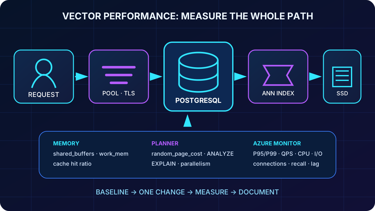
• Measure query latency, recall, QPS, cache hit ratio, CPU, memory, storage I/O, connections, and replica lag.
• Tune PostgreSQL memory and planner behavior.
• Choose and configure ANN indexes from data size, update pattern, accuracy, and build budget.
• Improve vector and metadata layout, then scale compute, reads, cache, and connections only where evidence points.

Topic summary

Start from an explicit latency and recall objective, a production-like baseline, and measurements across the full request path.

radio_button_uncheckedshort_text2. Understand the cost of vector distance

A 1,536-dimension comparison performs work across every element; an exact scan over one million rows therefore implies more than 1.5 billion element-level operations. L2 (<->) also computes a square root. Cosine distance (<=>) normalizes magnitude and is a common semantic default. Negative inner product (<#>) is usually the lightest calculation, but it represents similarity correctly only when the model produces—or the application stores—normalized vectors.

Doubling the dimension doubles vector storage and substantially increases distance work. Test whether 768 or 1,024 dimensions preserves product quality before paying for 1,536 or 3,072. For two million 1,536-dimensional vectors, raw vectors alone approach 12 GB; an HNSW graph can add roughly half again or more, depending on configuration and data.

Topic summary

Metric and dimension choices affect both relevance and the amount of CPU, memory, and storage consumed by every search.

radio_button_uncheckedshort_text3. Tune memory without multiplying risk

shared_buffers is PostgreSQL’s own page cache. A practical initial value is around one quarter of available memory, but Azure presets and workload evidence take precedence. For vector-heavy access, investigate a cache hit ratio below about 99%. work_mem is allocated per sort or hash operation and potentially several times per connection; setting 256 MB globally across hundreds of sessions can exhaust memory, so prefer SET LOCAL for exceptional searches.

effective_cache_size does not reserve memory; it tells the planner how much PostgreSQL plus operating-system cache is likely available. A value near 75% of memory is a common dedicated-server starting estimate. It can make index access look more attractive, but must reflect the deployed tier.

-- Inspect memory and planner settings
SHOW shared_buffers;
SHOW work_mem;
SHOW effective_cache_size;
SHOW random_page_cost;
SHOW effective_io_concurrency;

-- Change expensive settings only for the current transaction
BEGIN;
SET LOCAL work_mem = '256MB';
SET LOCAL hnsw.ef_search = 100;
-- run the vector query here
COMMIT;

SELECT
  sum(heap_blks_hit)::numeric /
  nullif(sum(heap_blks_hit + heap_blks_read), 0) AS cache_hit_ratio
FROM pg_statio_user_tables;

EXPLAIN (ANALYZE, BUFFERS)
SELECT id, title
FROM products
WHERE category_id = $2
ORDER BY embedding <=> $1::vector
LIMIT 10;

Topic summary

Keep the vector working set hot, size planner expectations realistically, and scope large work_mem values to transactions instead of every connection.

radio_button_uncheckedshort_text4. Align the planner and SSD I/O settings

The historical random_page_cost default of 4.0 models spinning disks. Managed SSD storage commonly warrants a measured starting range around 1.1–1.5 so random index access is not unfairly penalized. effective_io_concurrency around 200 can help supported SSD workloads prefetch blocks, especially for bitmap scans combined with metadata filters.

For exact scans or queries that cannot use an ANN index, more max_parallel_workers_per_gather and lower parallel_setup_cost or parallel_tuple_cost can encourage parallel plans. Do not force parallelism blindly: inspect EXPLAIN (ANALYZE, BUFFERS), actual versus estimated rows, Index Scan versus Seq Scan, and run ANALYZE after large changes. Azure Monitor should confirm that an apparent SQL improvement did not merely shift pressure to CPU or I/O.

Topic summary

Planner costs should describe SSD-backed Azure resources, while query plans and platform metrics verify the result.

radio_button_uncheckedshort_text5. Decide when approximate indexing pays off

An ANN index can improve speed by orders of magnitude but sacrifices some recall. Always compare returned neighbors with an exact-search reference set. Exact search remains appropriate for tiny tables, a highly selective prefilter, legally exact nearest-neighbor requirements, or data that changes too fast to keep an index useful.

Topic summary

Use ANN when scan cost dominates, but keep an exact baseline to quantify the recall exchanged for latency.

radio_button_uncheckedshort_text6. Configure IVFFlat for fast builds and controlled recall

IVFFlat clusters representative vectors into lists and probes only some lists at query time. It builds quickly and uses less memory than HNSW, which suits constrained servers, 90–95% recall targets, development, and catalogs refreshed in large batches. It needs data before training and can require rebuilding after a major distribution shift.

Lists guidance is deliberately heuristic: around 100 up to 100,000 rows, around 1,000 near one million, and several thousand for multi-million sets. For two million products, benchmark roughly 1,500–2,000 as one starting experiment alongside broader list counts. Start probes near sqrt(lists), or roughly 5–10% of lists for a recall-oriented test, then choose from the measured latency/recall curve.

-- IVFFlat: build after representative rows are loaded
CREATE INDEX CONCURRENTLY products_embedding_ivf_idx
ON products USING ivfflat (embedding vector_cosine_ops)
WITH (lists = 2000);

SET LOCAL ivfflat.probes = 45;

-- HNSW: higher memory and build cost, usually stronger recall/latency
CREATE INDEX CONCURRENTLY products_embedding_hnsw_idx
ON products USING hnsw (embedding vector_cosine_ops)
WITH (m = 16, ef_construction = 64);

SET LOCAL hnsw.ef_search = 100;

Topic summary

IVFFlat favors build speed and memory efficiency; lists shape the clusters and probes control query-time recall and work.

radio_button_uncheckedshort_text7. Configure HNSW—and know when DiskANN fits

HNSW navigates a multilayer proximity graph. Start m near 16; 32 can improve connectivity at extra memory cost. ef_construction must be at least 2 × m and often starts near 4 × m for a stronger graph. At query time, ef_search defaults around 40; latency-sensitive calls may test 20, while high-recall calls often test 100–200. Keep ef_search at least as large as LIMIT.

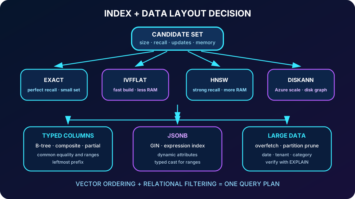
Choose HNSW for read-heavy workloads, ample RAM, small continuous inserts, and recall near 99% when longer builds are acceptable. Azure’s DiskANN is another large-scale option with high recall, fast query behavior, product quantization, and support for very high dimensions in recent versions. Confirm extension version and feature availability for the target server.

Topic summary

HNSW spends memory and build time for recall and latency; DiskANN extends the choice for Azure-scale and high-dimensional workloads.

radio_button_uncheckedshort_text8. Build, verify, and maintain vector indexes

The operator class must match the query operator: vector_cosine_ops with <=>, vector_l2_ops with <->, and vector_ip_ops with <#>. A mismatch is a common reason for a sequential scan. Load representative data before IVFFlat, create production indexes concurrently, update statistics, and prove use with EXPLAIN ANALYZE.

Illustrative—not guaranteed—build windows can range from minutes for IVFFlat over one million rows to hours for HNSW over ten million rows. Hardware, storage, parallelism, m, ef_construction, lists, and data shape dominate. Track progress and scan counts, then use concurrent reindexing when distribution drift or bloat justifies it.

SELECT phase,
       round(100.0 * blocks_done / nullif(blocks_total, 0), 1) AS percent
FROM pg_stat_progress_create_index;

SELECT indexrelname, idx_scan, idx_tup_read,
       pg_size_pretty(pg_relation_size(indexrelid)) AS size
FROM pg_stat_user_indexes
WHERE relname = 'products';

REINDEX INDEX CONCURRENTLY products_embedding_hnsw_idx;

Topic summary

Index creation is an observable production operation; matching operators, current statistics, progress, use counts, and rebuild policy all matter.

radio_button_uncheckedshort_text9. Design vectors and metadata for the queries you run

Declare vector dimensions explicitly so incompatible embeddings fail early. Separate title, image, and behavior embeddings when they represent distinct spaces, and build an index for each queried vector. Put stable, frequently filtered fields in native typed columns; reserve JSONB for dynamic, nested, or rarely filtered attributes.

B-tree indexes accelerate equality and ranges. Composite order follows the leftmost-prefix rule, and partial indexes are valuable for predicates such as in_stock. GIN supports JSONB containment and key operators; a numeric range extracted from JSONB usually needs an expression index so comparison is numeric, not textual.

CREATE TABLE products (
  id BIGSERIAL PRIMARY KEY,
  category_id BIGINT NOT NULL,
  price NUMERIC(12,2) NOT NULL,
  in_stock BOOLEAN NOT NULL,
  attributes JSONB NOT NULL DEFAULT '{}',
  title_embedding vector(768),
  image_embedding vector(512)
);

CREATE INDEX products_category_price_idx
  ON products(category_id, price);
CREATE INDEX products_available_category_idx
  ON products(category_id) WHERE in_stock;
CREATE INDEX products_attributes_gin_idx
  ON products USING gin(attributes);
CREATE INDEX products_attribute_price_idx
  ON products (((attributes->>'price')::numeric));

Topic summary

Use one explicit vector space per purpose, typed columns for common predicates, JSONB for flexibility, and indexes that match actual filters.

radio_button_uncheckedshort_text10. Combine metadata filtering with vector search

A category that selects 5% of a two-million-row catalog reduces potential distance work to about 100,000 rows. PostgreSQL may lead with the metadata index when the filter is selective or with the vector index when it is broad. EXPLAIN ANALYZE tells you which path won.

ANN systems can apply a predicate after retrieving candidates. If you need ten final rows, retrieve more than ten and filter the candidates; size that overfetch from observed selectivity. Too little returns incomplete results, while too much wastes the ANN gain.

-- Let PostgreSQL combine a selective metadata filter with vector ordering
SELECT id, title
FROM products
WHERE category_id = $2 AND in_stock
ORDER BY embedding <=> $1::vector
LIMIT 10;

-- If filtering occurs after ANN retrieval, deliberately overfetch
WITH candidates AS (
  SELECT id, title, category_id, in_stock,
         embedding <=> $1::vector AS distance
  FROM products
  ORDER BY embedding <=> $1::vector
  LIMIT 100
)
SELECT * FROM candidates
WHERE category_id = $2 AND in_stock
ORDER BY distance LIMIT 10;

Topic summary

Selective metadata indexes shrink vector work; post-filter designs must overfetch deliberately and be checked with real plans.

radio_button_uncheckedshort_text11. Partition only when it matches data access

At tens of millions of rows, partitioning can prune irrelevant dates, tenants, or categories, let teams drop old data cheaply, and keep index maintenance bounded. Range fits time, list fits a small set of categories, and hash spreads tenants or keys. Creating an index on the parent creates corresponding partition indexes.

CREATE TABLE product_vectors (
  id BIGINT, created_at TIMESTAMPTZ NOT NULL, embedding vector(1536)
) PARTITION BY RANGE (created_at);

CREATE TABLE product_vectors_2026_08
PARTITION OF product_vectors
FOR VALUES FROM ('2026-08-01') TO ('2026-09-01');

CREATE INDEX ON product_vectors
USING hnsw (embedding vector_cosine_ops);

Partitioning also adds cross-partition planning, unique constraints that must include the partition key, and application/operations complexity. It is useful only when important queries carry the partition key and pruning is visible in the plan.

Topic summary

Partition for a natural access boundary at large scale, not as a substitute for a good schema and correct indexes.

radio_button_uncheckedshort_text12. Scale compute from the working set and concurrency

As starting hypotheses, test General Purpose with 4–8 vCores below one million vectors and consider Memory Optimized with 8–16 vCores for one to ten million. Hundreds of concurrent searches can need 32 or more. Scale vertically when one query needs more CPU, memory, or I/O; scale reads when aggregate QPS—not single-query execution—is the limit. Sustained CPU above roughly 70%, low cache residency, or I/O saturation are stronger signals than row count alone.

Topic summary

Choose the tier from working-set memory, single-query cost, concurrency, and measured saturation rather than a fixed row-count formula.

radio_button_uncheckedshort_text13. Distribute reads and cache repeatable results

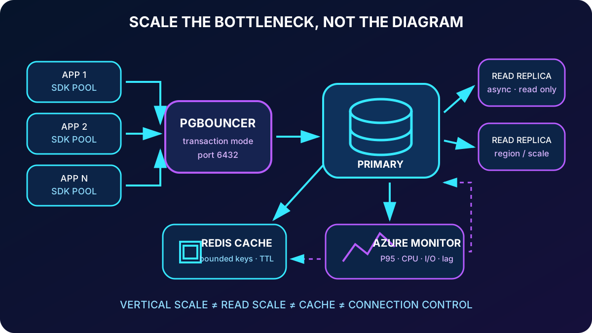
Read replicas use asynchronous physical streaming and have their own endpoint, region, and size. They fit recommendation and semantic-read traffic that tolerates brief staleness; route just-updated preferences or read-after-write paths to the primary. Monitor replay lag, because bulk writes, network delay, or an undersized replica can expand it. Current Azure documentation supports replicas on General Purpose and Memory Optimized, not Burstable.

Cache popular product embeddings, precomputed similar-item lists, stable user embeddings, and category aggregates. Arbitrary query vectors, rapidly changing values, and combinations with huge key cardinality are poor cache candidates. Start recommendation TTLs around 15–60 minutes, then use event invalidation or background refresh where freshness matters.

SELECT now() - pg_last_xact_replay_timestamp() AS replica_lag;

# Cache a bounded, repeatable recommendation result
SETEX recommendations:product:4281 1800 '{"ids":[18,77,304]}'

The source module names Azure Cache for Redis. Microsoft has since announced its retirement and recommends Azure Managed Redis for new designs and migration planning; preserve the cache pattern while choosing the current service.

Topic summary

Replicas add read throughput with possible lag; Redis caching removes repeated work when keys are bounded and freshness is managed.

radio_button_uncheckedshort_text14. Monitor capacity, growth, and cost together

Track CPU percentage, memory percentage, storage I/O, active connections, P95/P99 latency, QPS, recall, cache hit rate, and replica lag. Example operational thresholds might warn after CPU exceeds 80% for five minutes and escalate when memory passes 90%, but baselines and service objectives determine the real values.

1. Capture the present baseline and peak window.
2. Project catalog, embedding dimension, update rate, QPS, and concurrency growth.
3. Load-test production-like vectors and filters.
4. Document the condition that triggers a larger tier, replica, cache, index rebuild, or partition.
5. Review after model or traffic changes instead of waiting for an incident.

Reduce cost when CPU remains below roughly 30% and headroom is excessive. Evaluate reservations for steady baseline capacity, keep burst capacity flexible, remove unused indexes, archive obsolete vectors, use the lowest precision that passes quality tests, and keep Burstable for development rather than a latency SLO it cannot sustain.

Topic summary

Capacity planning joins performance telemetry, growth forecasts, trigger thresholds, and cost controls in one repeatable loop.

radio_button_uncheckedshort_text15. Pool database connections with PgBouncer

Opening a connection can consume 50–200 ms across TCP, TLS, authentication, a PostgreSQL backend, and session initialization. Maximum connections vary by tier and size and can change; treat figures such as 859 for a small General Purpose server or about 5,000 for larger servers as examples, not contracts. Query the deployed service limits.

Built-in PgBouncer is available for General Purpose and Memory Optimized and listens on port 6432. Transaction mode is the normal vector-API choice: a server connection returns to the pool after commit or rollback. Session mode retains all session features but reduces less; statement mode maximizes reuse but cannot support multi-statement transactions.

# Built-in PgBouncer endpoint uses port 6432
postgresql://app@server:password@server.postgres.database.azure.com:6432/appdb

# Suggested starting posture; benchmark for the real workload
pool_mode = transaction
default_pool_size = 40
max_client_conn = 5000
query_wait_timeout = 60

Transaction pooling does not preserve ordinary SET state; use SET LOCAL or server defaults. Named prepared statements can be tied to a backend, and LISTEN/NOTIFY is incompatible with transaction pooling. Begin around 20–50 server connections per pool, leave headroom, and benchmark rather than copying a maximum.

Topic summary

PgBouncer amortizes connection setup and protects server limits; transaction mode is efficient when code avoids session-dependent behavior.

radio_button_uncheckedshort_text16. Combine SDK pools, batching, async I/O, and resilience

An application pool reduces local connection churn before PgBouncer. If a server safely allows 1,000 backends and ten application instances share it, an upper bound near 100 per instance still needs headroom for operations and failover. Too-small pools queue every request; too-large pools convert application concurrency into database overload. Recycle connections after roughly 30–60 minutes and use consistent connection strings so .NET does not fragment Npgsql pools.

from psycopg_pool import AsyncConnectionPool

pool = AsyncConnectionPool(
    conninfo=DATABASE_URL,
    min_size=5,
    max_size=20,
    max_idle=300,
    max_lifetime=3600,
)

async with pool.connection() as conn:
    async with conn.transaction():
        await conn.execute("SET LOCAL hnsw.ef_search = 100")
        rows = await conn.execute(
            "SELECT id FROM products ORDER BY embedding <=> %s LIMIT 10",
            (query_vector,),
        )

Batch IDs with ANY rather than a query per row, and use COPY for large ingestion. Async tasks improve throughput while waiting for network/database I/O, but concurrency must remain under pool limits. Configure connect and statement timeouts, catch pool timeouts as controlled overload, and retry transient OperationalError failures only a few times with exponential backoff plus jitter.

Topic summary

A bounded SDK pool, PgBouncer, set-local tuning, bulk operations, async I/O, timeouts, and finite jittered retries form one connection strategy.

radio_button_uncheckedshort_text17. Guided lab: optimize a PostgreSQL vector search

The source exercise is designed for about 30 minutes and turns the principles into a controlled comparison.

1. Prepare an Azure subscription, Visual Studio Code, the latest Azure CLI, and psql.
2. Download the starter files and review the deployment configuration.
3. Deploy an Azure Database for PostgreSQL flexible server with Microsoft Entra authentication.
4. Generate a test dataset with embeddings.
5. Record an exact-search baseline and its plan.
6. Build IVFFlat and HNSW indexes, then compare latency and recall against the exact result.
7. Tune lists/probes or m/ef values one at a time, capture the result, and remove disposable resources.

Topic summary

The lab produces a repeatable exact baseline, two ANN experiments, and a documented speed-versus-recall decision.

radio_button_uncheckedshort_text18. Assessment review and production checklist

1. With two million 1,536-dimensional vectors and an 85% cache hit ratio, first increase or right-size shared_buffers and verify the working set.
2. For five million embeddings replaced in a daily full refresh under a short build window, IVFFlat with a row-informed list count fits better than HNSW.
3. When category-filtered vector search performs a sequential scan, first confirm a B-tree index on category_id, then also verify the vector operator class and statistics.
4. At 500 vector queries per second, use PgBouncer transaction mode with a pool sized across application instances instead of opening one connection per request.
5. For a CPU-bound General Purpose server at 75% and a single-query P95 target below 50 ms, test a larger Memory Optimized tier before replicas or cache, because they do not accelerate the uncached individual query.

• Baseline latency, recall, QPS, hit ratio, CPU, I/O, and connections.
• Keep vector dimensions and distance/operator classes consistent.
• Verify metadata and ANN plans with EXPLAIN ANALYZE.
• Watch index builds, usage, drift, bloat, and replay lag.
• Use current Azure Redis guidance, bounded pools, transaction-safe settings, timeouts, and controlled retries.
• Document thresholds and reassess after every material model, catalog, or traffic change.

Official references

1. Optimize pgvector performance in Azure Database for PostgreSQL
2. Enable and use DiskANN
3. Read replicas in Azure Database for PostgreSQL flexible server
4. Built-in PgBouncer in Azure Database for PostgreSQL
5. Migrate Azure Cache for Redis to Azure Managed Redis

Topic summary

Production vector performance comes from evidence-driven tuning across compute, data, indexes, distribution, cache, and connections—not one magic parameter.