Implement vector search and RAG with PostgreSQL and pgvector

radio_button_uncheckedshort_text1. Turn an existing PostgreSQL database into an AI retriever

Suppose a legal knowledge system already keeps document metadata and client records in Azure Database for PostgreSQL. Attorneys need to find cases, clauses, and precedents by meaning—even when their query and the source use different wording. Keeping embeddings beside the relational data avoids another vector service and a synchronization pipeline, while still supporting new documents every day and sub-second retrieval at scale.

• Store and query embeddings with pgvector.
• Choose a distance metric and execute similarity queries.
• Select and tune approximate nearest-neighbor indexes.
• Refresh vectors and migrate embedding models safely.
• Build semantic, hybrid, and RAG retrieval with citations and measurable quality.

Topic summary

pgvector adds semantic retrieval to the PostgreSQL data already used by an application, reducing architecture and synchronization overhead.

radio_button_uncheckedshort_text2. Enable pgvector and design vector-aware schemas

On Azure Database for PostgreSQL flexible server, first allow the extension at server scope, confirm the setting with SHOW azure.extensions, and then create it in every database that needs it. The community name is pgvector, but the binary and SQL extension name are vector. Creating it normally requires the server administrator or a member of azure_pg_admin.

CREATE EXTENSION IF NOT EXISTS vector;

CREATE TABLE knowledge_chunks (
  id BIGSERIAL PRIMARY KEY,
  source_id BIGINT NOT NULL,
  chunk_no INTEGER NOT NULL,
  title TEXT NOT NULL,
  content TEXT NOT NULL,
  category TEXT,
  token_count INTEGER,
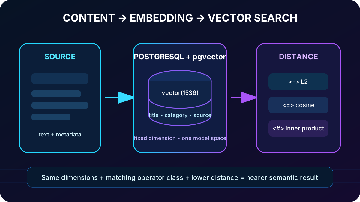
  embedding vector(1536),
  embedding_stale BOOLEAN NOT NULL DEFAULT false,
  updated_at TIMESTAMPTZ NOT NULL DEFAULT now(),
  UNIQUE (source_id, chunk_no)
);

The dimension in vector(n) must exactly match the embedding model output. A 384-dimension sentence model, a 1,536-dimension model, and a model capable of 3,072 dimensions cannot share one constrained column unless their outputs are transformed to the same size. Keep useful filter and display metadata with each vector; move very large bodies to another table only when reducing retrieval traffic justifies the join.

Use separate vector columns when title and body embeddings or multiple models serve different retrieval signals. Standard INSERT, multi-row INSERT, or COPY can load vectors, and a content update must eventually regenerate the corresponding embedding.

Topic summary

Allow and create the vector extension per database, then bind each vector column to the exact dimension and retrieval purpose of one embedding space.

radio_button_uncheckedshort_text3. Choose vector, halfvec, or sparsevec intentionally

For dense embeddings from common text models, begin with vector. Benchmark halfvec before adopting it, because cheaper storage is not useful if relevance falls below the product target. HNSW indexing of sparsevec supports at most 1,000 nonzero elements; reduce dimensions or choose another strategy when the sparse representation exceeds that limit.

Topic summary

Use vector by default, halfvec only after quality testing, and sparsevec for genuinely sparse representations within index limits.

radio_button_uncheckedshort_text4. Match distance operators to the embedding model

-- Euclidean/L2: smaller means nearer
SELECT id, title, embedding <-> $1::vector AS distance
FROM knowledge_chunks ORDER BY embedding <-> $1::vector LIMIT 8;

-- Cosine distance: common for text embeddings
SELECT id, title, embedding <=> $1::vector AS distance
FROM knowledge_chunks ORDER BY embedding <=> $1::vector LIMIT 8;

-- Negative inner product: smaller means a larger dot product
SELECT id, title, embedding <#> $1::vector AS distance
FROM knowledge_chunks ORDER BY embedding <#> $1::vector LIMIT 8;

Lower is better for all three operators as exposed by pgvector. Confirm the recommendation of the embedding model rather than choosing from habit. Normalized vectors can make inner product especially efficient, while cosine distance is a frequent text-search default. Parameterize vectors instead of concatenating them into SQL.

Topic summary

The distance operator must match the model geometry; pgvector orders all three distance results from smaller to more similar.

radio_button_uncheckedshort_text5. Understand exact search, ANN, recall, and DiskANN

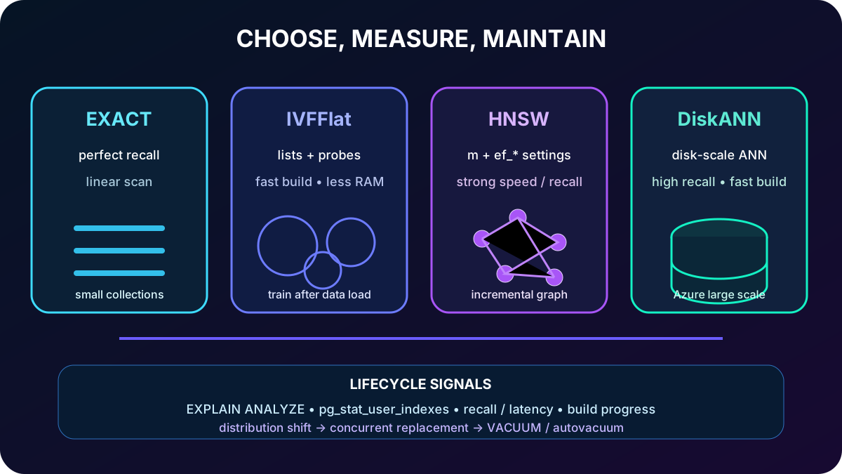
Without an index, PostgreSQL compares the query with every row and returns the true nearest neighbors. That exact scan guarantees perfect recall but grows linearly; it can be reasonable below roughly ten thousand rows and increasingly costly at hundreds of thousands or millions.

Approximate nearest-neighbor search examines a structured subset. Its quality is expressed as recall: the fraction of the exact neighbors that also appear in the approximate result. Many AI systems accept 95–99% recall in exchange for millisecond latency. Azure Database for PostgreSQL also supports DiskANN through pg_diskann, providing high recall and throughput with disk-oriented scaling, fast builds, product quantization, and—on recent versions—higher-dimensional indexing than pgvector HNSW/IVFFlat.

Topic summary

Exact search maximizes recall; ANN indexes trade a small amount of recall for large latency gains, with DiskANN adding an Azure-optimized large-scale option.

radio_button_uncheckedshort_text6. Build and tune IVFFlat

IVFFlat runs k-means at index creation and divides vectors into lists around centroids. A query finds the closest centroids and searches only the number of lists selected by probes. Approximate work is therefore proportional to (rows / lists) × probes rather than the entire table.

• Load representative data before creating the index; an empty table cannot train useful clusters.
• For up to about one million rows, a starting lists estimate is rows / 1,000; for larger sets, start near the square root of the row count.
• Start probes near sqrt(lists). Raising it improves recall and increases latency.
• Rebuild when a large or semantically different data arrival makes the original clusters unrepresentative.

Topic summary

IVFFlat is memory-efficient and quick to build, but depends on representative training data and a lists/probes balance.

radio_button_uncheckedshort_text7. Build and tune HNSW

HNSW creates a multi-layer proximity graph. A query begins in a sparse upper layer, follows promising links, and descends into denser layers until it reaches candidates near the query. Unlike IVFFlat, it can start on an empty table and evolve with inserts.

CREATE INDEX chunks_embedding_hnsw_idx
ON knowledge_chunks USING hnsw (embedding vector_cosine_ops)
WITH (m = 16, ef_construction = 96);

SET LOCAL hnsw.ef_search = 100;

-- Alternative after representative data exists
CREATE INDEX chunks_embedding_ivfflat_idx
ON knowledge_chunks USING ivfflat (embedding vector_cosine_ops)
WITH (lists = 100);

SET LOCAL ivfflat.probes = 10;

m limits graph connections per node: increasing it can improve recall but costs memory and build time. ef_construction widens candidate search during index creation; higher values usually improve graph quality while slowing the build. ef_search widens query-time exploration; start from the default and raise it only when measured recall requires it.

Topic summary

HNSW generally delivers stronger speed/recall behavior, paid for with more memory, slower construction, and moderate insert overhead.

radio_button_uncheckedshort_text8. Choose the index and prove that PostgreSQL uses it

Choose HNSW when low latency and high recall dominate and memory is available. Choose IVFFlat when builds, memory, or frequent bulk refreshes matter more. The operator class must match the query: vector_l2_ops with <->, vector_cosine_ops with <=>, and vector_ip_ops with <#>. A mismatch prevents the vector index from satisfying the ordering.

EXPLAIN (ANALYZE, VERBOSE, BUFFERS)
SELECT id, title
FROM knowledge_chunks
ORDER BY embedding <=> $1::vector
LIMIT 10;

Expect an Index Scan for a sufficiently large table and an ORDER BY distance with LIMIT. A Seq Scan can still be rational on a small table. Also confirm that the index is valid, statistics are current, and the LIMIT is present.

Topic summary

Pick from workload evidence, match operator class to operator, and verify the execution plan rather than assuming the index is active.

radio_button_uncheckedshort_text9. Monitor, rebuild, and reclaim vector storage

pg_stat_user_indexes reveals scan counts and index size; zero scans can expose a mismatched operator or planner choice. Track representative EXPLAIN ANALYZE latency and retrieval recall over time. pg_stat_progress_create_index exposes build phases and progress, especially while tuples are loading.

Rising latency without equivalent data growth, falling result quality, or roughly 20–30% new data from a different domain are rebuild signals. For continuous service, build a replacement with CREATE INDEX CONCURRENTLY, validate it, drop the old one, and rename the replacement. REINDEX is simpler when a write interruption is acceptable.

Estimate vector storage as dimensions × 4 bytes × rows for vector, then add index overhead—often about 1.5–2× vector size for HNSW and 1–1.5× for IVFFlat. PostgreSQL MVCC leaves dead tuples after updates. VACUUM reclaims reusable space; VACUUM FULL returns more disk space but locks the table. Heavy-refresh tables may need lower autovacuum scale factors.

Topic summary

Use system statistics, query plans, recall checks, concurrent replacement, and vacuum policy to keep vector structures healthy.

radio_button_uncheckedshort_text10. Refresh embeddings without blocking content writes

An embedding is stale as soon as its source meaning changes. Occasional updates can generate the vector and commit content plus embedding atomically, but that couples write latency to the embedding endpoint. Frequent change is better handled asynchronously: flag stale rows, have workers claim bounded batches, generate embeddings in bulk, and clear the flag only after the vector is stored.

-- Content writes stay fast and mark the vector as stale
UPDATE knowledge_chunks
SET content = $1, embedding_stale = true, updated_at = now()
WHERE id = $2;

-- A worker claims a bounded batch without colliding with peers
SELECT id, content
FROM knowledge_chunks
WHERE embedding_stale
ORDER BY updated_at
FOR UPDATE SKIP LOCKED
LIMIT 250;

-- The worker writes the regenerated vector
UPDATE knowledge_chunks
SET embedding = $1::vector, embedding_stale = false
WHERE id = $2;

A scheduled full refresh can catch missed changes and normalize a dataset after settings evolve. Process older rows first, respect API rate limits, keep transactions in manageable batches—often 1,000 to 5,000 updates for a large backfill—and monitor replication, locks, WAL, and index growth.

Topic summary

Use atomic refresh for rare edits and stale flags plus batch workers for high-change corpora and resilient embedding generation.

radio_button_uncheckedshort_text11. Migrate embedding models with parallel columns

Vectors from different models or dimensions do not belong in the same search space. Overwriting the active column during a migration mixes incompatible semantics and produces unstable results. Add a second column, create its matching index, backfill in batches, compare both versions on a labeled evaluation set, switch reads atomically, and retain the old path until rollback is no longer required.

ALTER TABLE knowledge_chunks ADD COLUMN embedding_v2 vector(3072);

CREATE INDEX CONCURRENTLY chunks_embedding_v2_idx
ON knowledge_chunks USING hnsw (embedding_v2 vector_cosine_ops);

-- Backfill in bounded batches, compare recall and latency, then switch reads.
-- Keep the original column until the new model passes acceptance tests.

Estimate time from row count, batch throughput, embedding API quotas, and retry rate. Temporary storage includes both columns and both indexes, so capacity must be planned before the migration begins.

Topic summary

A parallel-column migration avoids mixed vector spaces, supports quality comparison, and preserves a rollback path.

radio_button_uncheckedshort_text12. Combine semantic retrieval with metadata and quality thresholds

SELECT id, title, content, category,
       embedding <=> $1::vector AS distance
FROM knowledge_chunks
WHERE category = $2
  AND embedding <=> $1::vector < $3
ORDER BY embedding <=> $1::vector
LIMIT $4;

B-tree indexes on frequent metadata filters—sometimes composite indexes—can shrink the candidate set. The planner may favor metadata indexes for very selective predicates or the vector index for broad filters; ANALYZE and EXPLAIN ANALYZE show the actual decision.

LIMIT alone always returns N rows, even when none are useful. A distance threshold establishes a quality floor and can correctly return nothing. Derive it from labeled relevant and irrelevant query/document pairs rather than copying a universal number. Retrieve title, content, citation metadata, and distance in one round trip, while avoiding full-text transfer when a summary is sufficient.

Topic summary

Metadata filters control scope, thresholds control minimum relevance, and query plans reveal how PostgreSQL combines relational and vector access.

radio_button_uncheckedshort_text13. Handle multi-vector and hybrid searches

Average example vectors when they express one coherent concept from several angles. Keep separate vectors when the query has independent requirements—such as merger law and environmental compliance—then retrieve candidates for each aspect and combine their evidence.

Vector similarity captures meaning but can underweight exact case names, product codes, or technical terms. PostgreSQL full-text search supplies lexical ranking and a GIN index can accelerate a stored or generated tsvector. Hybrid retrieval joins semantic and lexical candidates. Reciprocal Rank Fusion (RRF) combines rank positions without pretending that vector distance and text relevance share the same numeric scale.

WITH semantic AS (
  SELECT id, row_number() OVER (ORDER BY embedding <=> $1::vector) AS rank
  FROM knowledge_chunks ORDER BY embedding <=> $1::vector LIMIT 40
), lexical AS (
  SELECT id, row_number() OVER (
    ORDER BY ts_rank_cd(to_tsvector('simple', content), websearch_to_tsquery('simple', $2)) DESC
  ) AS rank
  FROM knowledge_chunks
  WHERE to_tsvector('simple', content) @@ websearch_to_tsquery('simple', $2)
  LIMIT 40
)
SELECT k.id, k.title,
       coalesce(1.0 / (60 + s.rank), 0) + coalesce(1.0 / (60 + l.rank), 0) AS rrf_score
FROM knowledge_chunks k
LEFT JOIN semantic s ON s.id = k.id
LEFT JOIN lexical l ON l.id = k.id
WHERE s.id IS NOT NULL OR l.id IS NOT NULL
ORDER BY rrf_score DESC LIMIT 10;

Topic summary

Use averaged vectors for one concept, separate retrieval for distinct concepts, and RRF when semantic meaning and exact terms both matter.

radio_button_uncheckedshort_text14. Design a RAG document-and-chunk model

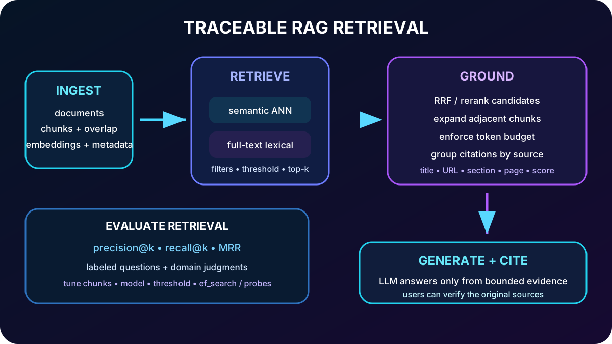
RAG converts a question to an embedding, retrieves relevant evidence, and asks a language model to answer from that evidence. Retrieval quality therefore bounds generation quality. Whole documents are often too broad or too large, so separate source metadata from independently searchable chunks.

CREATE TABLE source_documents (
  id BIGSERIAL PRIMARY KEY,
  title TEXT NOT NULL,
  source_url TEXT,
  document_type TEXT,
  version INTEGER NOT NULL DEFAULT 1,
  ingested_at TIMESTAMPTZ NOT NULL DEFAULT now()
);

CREATE TABLE document_chunks (
  id BIGSERIAL PRIMARY KEY,
  document_id BIGINT NOT NULL REFERENCES source_documents(id) ON DELETE CASCADE,
  chunk_no INTEGER NOT NULL,
  section_title TEXT,
  page_number INTEGER,
  content TEXT NOT NULL,
  token_count INTEGER NOT NULL,
  embedding vector(1536),
  UNIQUE (document_id, chunk_no)
);

CREATE INDEX chunks_source_order_idx ON document_chunks(document_id, chunk_no);

Store section, page, offsets, and token counts so retrieval can rebuild context and citations. Batch embedding requests and chunk inserts to reduce round trips. Replacing a document can cascade-delete old chunks before reingestion; versioned domains can keep multiple editions and filter the active version.

Topic summary

Separate documents from chunks, preserve traceability metadata, and choose chunk boundaries from corpus structure and question patterns.

radio_button_uncheckedshort_text15. Build context windows, token budgets, and citations

Top-k retrieval works when chunks are self-contained. Narrative or cross-referencing content often needs adjacent chunks around each match. Expand only within the same document, deduplicate overlaps, and track cumulative tokens so the system leaves room for instructions, the user question, and the generated answer.

WITH seeds AS (
  SELECT id, document_id, chunk_no, embedding <=> $1::vector AS distance
  FROM document_chunks
  ORDER BY embedding <=> $1::vector
  LIMIT 4
), expanded AS (
  SELECT DISTINCT c.*, s.distance
  FROM seeds s
  JOIN document_chunks c ON c.document_id = s.document_id
   AND c.chunk_no BETWEEN s.chunk_no - 1 AND s.chunk_no + 1
), budgeted AS (
  SELECT e.*, d.title, d.source_url,
         sum(e.token_count) OVER (ORDER BY e.distance, e.chunk_no) AS tokens_used
  FROM expanded e JOIN source_documents d ON d.id = e.document_id
)
SELECT content, title, source_url, section_title, page_number, distance
FROM budgeted WHERE tokens_used <= 3200
ORDER BY distance, chunk_no;

Return source title, stable URL or ID, section, page, and distance. Group several matching chunks from one source into one citation with multiple excerpts instead of flooding the response with duplicates. High-stakes domains should make every claim verifiable and flag weak matches for human review.

Topic summary

Expand context only where needed, enforce a token budget, and return enough metadata for a user to verify every source.

radio_button_uncheckedshort_text16. Evaluate retrieval separately from generation

Build an evaluation set from about 20–50 representative questions to start, retrieve 10–20 candidates, and have a domain expert label relevance. Automate precision@k, recall@k, and MRR so changes to models, chunk size, overlap, thresholds, and index parameters can be compared rather than guessed. Smaller chunks can sharpen precision but fragment facts; overlap improves continuity but duplicates storage; broader ANN search improves recall but adds latency.

Topic summary

A labeled query set and retrieval metrics make model, chunking, threshold, and index tuning evidence-driven.

radio_button_uncheckedshort_text17. Guided lab: product similarity with Flask

The source exercise allocates about 30 minutes to build a product-similarity web app, a reusable pattern for recommendations, semantic search, and RAG retrieval.

1. Prepare an Azure subscription with deployment rights, Visual Studio Code, the latest Azure CLI, Python 3.12 or later, and psql.
2. Download the starter project and configure the deployment script.
3. Deploy an Azure Database for PostgreSQL flexible server with Microsoft Entra authentication.
4. Complete the Flask application while the server deployment runs.
5. Allow and enable vector, then create the products table with its embedding column.
6. Load sample products, run similarity searches, and inspect ordering and distances.
7. Add products and observe how the neighborhood changes.
8. Remove disposable Azure resources after validation.

Topic summary

The lab connects secure provisioning, pgvector schema creation, Flask ingestion, and live similarity results in one working flow.

radio_button_uncheckedshort_text18. Assessment review and final checklist

1. For semantic similarity with unit-normalized embeddings, cosine distance (<=>) is the expected assessment answer; model guidance can also justify inner product in optimized implementations.
2. For five million embeddings with occasional batch updates and no real-time inserts, IVFFlat with suitable lists is the assessment choice because its build and memory profile fit that scenario.
3. In HNSW, m controls the maximum connections per graph node; ef_construction controls candidate exploration during the build.
4. For 50,000 regenerated product vectors, bounded transactions of roughly 1,000–5,000 rows reduce disruption compared with one giant transaction.
5. RRF balances hybrid rankings without directly multiplying incomparable semantic and lexical scores.

• Match dimension, model, operator, and operator class.
• Measure recall and latency before choosing exact, HNSW, IVFFlat, or DiskANN.
• Monitor plans, scan counts, build progress, bloat, and data-distribution changes.
• Refresh asynchronously when content changes frequently and migrate models with parallel columns.
• Filter and threshold semantic search, add lexical evidence when exact terms matter.
• Design RAG for chunk integrity, token limits, citations, and measurable retrieval quality.

Official references

1. Enable and use pgvector in Azure Database for PostgreSQL flexible server
2. Optimize performance when using pgvector
3. Enable and use DiskANN
4. Integrate Azure AI capabilities with Azure Database for PostgreSQL
5. Create semantic search with Azure OpenAI

Topic summary

Production vector retrieval combines a consistent embedding space, verified indexes, maintainable refresh workflows, relational filters, and traceable RAG evidence.