Suggested study time: 36 minutes • Beginner level • Original rewrite based on Microsoft Learn objectives
By João Ricardo Dutra••Complete original content
1. Introduction to text analysis
Learning objectives
Explain how tokenization and preprocessing prepare a corpus for analysis.
Apply frequency, TF-IDF, bag-of-words, Naive Bayes, and TextRank conceptually.
Interpret embeddings, cosine similarity, vector arithmetic, and semantic relationships.
Connect semantic models with summarization, keywords, entities, classification, and sentiment.
Text analysis is a natural language processing, or NLP, discipline that extracts meaning, structure, and insight from unstructured text. Organizations use it to turn customer feedback, support tickets, contracts, and social media posts into actionable intelligence.
Methods have progressed from statistical term counts to vector language models that can represent meaning. This evolution addresses a core challenge: human language is complex, while computers require numerical representations to analyze it.
Common text-analysis workloads.
Task
Outcome
Language detection
Identifies one or more languages and often starts a multi-stage pipeline.
Key-term extraction
Finds important words and phrases to reveal themes.
Entity detection
Locates people, places, dates, organizations, and other named entities.
PII detection
Identifies and can redact names, addresses, phone numbers, financial accounts, and other sensitive data.
Text classification
Categorizes documents by content, such as spam versus non-spam.
Sentiment analysis
Classifies tone as positive, neutral, or negative.
Summarization
Reduces volume while retaining salient points.
Microsoft Learn offers the original material in video and text formats. The written version usually provides additional detail and can supplement the videos.
2. Tokenizing a corpus
The first analysis step is to split a collection of text, called a corpus, into tokens. For simplicity, every distinct word can be treated as a token, although real systems also use subwords, word combinations, and punctuation.
In “We choose to go to the moon,” every occurrence occupies a sequence position. The repeated “to” reuses its vocabulary identifier. This discrete representation makes frequencies easy to count and helps reveal dominant terms.
Simplified token sequence.
Position
Token
1
We
2
choose
3
to
4
go
5
to
6
the
7
moon
The best tokenization scheme depends on the problem. A solution may preserve capitalization and punctuation when they convey meaning, or remove them when the goal is simply to compare term frequency.
3. Normalization, stop words, and n-grams
Preprocessing techniques.
Technique
How it works
Trade-off
Normalization
May remove punctuation and convert text to lowercase.
Improves simple counts but can erase differences among the surname “Banks,” the noun “banks,” and a period that marks a sentence boundary.
Stop-word removal
Excludes functional words such as articles and pronouns that aid readability but carry little thematic meaning.
The list must fit the language and domain because a generally common word may still matter in context.
N-gram extraction
Groups recurring sequences. One word is a unigram, two form a bigram, and three form a trigram.
Phrases such as “artificial intelligence” and “natural language processing” should be treated as units when meaning depends on the combination.
4. Stemming, lemmatization, and part-of-speech tags
Stemming consolidates variants by stripping endings such as “s,” “ing,” and “ed.” The aim is to group terms with a shared root before counting them, even when the resulting stem is not a valid word.
Lemmatization also finds a base form, called a lemma, but applies linguistic rules and vocabulary. It therefore tends to return recognizable words, such as converting “running” to “run,” instead of merely cutting characters.
Part-of-speech, or POS, tagging labels tokens as nouns, verbs, adjectives, adverbs, and other grammatical categories. Linguistic rules and statistical models use both the token and its sentence context to choose the correct tag.
5. Frequency analysis
After tokenization, normalization, and lemmatization, a simple count shows how often each term occurs. The assumption is that recurring terms help identify a document’s themes.
In a passage about AI benefits in business, normalized counts might show “AI” four times, “business” three times, and “benefit,” “customer,” “decision,” and “market” twice each. The pattern points to business value from automation, predictive analytics, productivity, personalization, and market adaptation.
Partial frequency example after preprocessing.
Term
Frequency
AI
4
business
3
benefit
2
customer
2
decision
2
market
2
ability
1
accuracy
1
6. TF-IDF: relevance across documents
Raw frequency works for one document, but terms common throughout a corpus make documents difficult to distinguish. Term frequency-inverse document frequency, or TF-IDF, raises the weight of words that are frequent locally but rare across the collection.
Consider two agent-related samples. One presents declarative creation in Microsoft Copilot Studio through natural language, prompts, templates, intents, actions, data connections, channel publishing, orchestration, governance, and lifecycle management. The other describes code-first development in with SDKs, APIs, conversations, tool calling, state, pipelines, Python, C#, Microsoft AI services, and CI/CD.
“Agent,” “Microsoft,” and “AI” occur often in both samples and identify the broad topic without separating the documents. TF-IDF instead highlights “Copilot,” “Studio,” and “declarative” in the first, and “code,” “develop,” and “Foundry” in the second.
TF(t,d) = number of occurrences of t in document d
IDF(t) = log(N / df(t))
TF-IDF(t,d) = TF(t,d) × log(N / df(t))
N is the document count and df(t) is the number containing the term. A word in both documents when N = 2 has IDF log(2/2) = 0 and no discriminative weight. In the example, “copilot” and “studio” score 2.0794, “declarative” scores 1.3863; “code,” “develop,” and “foundry” score 2.0794 in the other sample.
7. Bag-of-words, Naive Bayes, and classification
Bag-of-words represents a document as a vector of token occurrences or frequencies while ignoring grammar and word order. Machine-learning algorithms can use this vector as input features.
Naive Bayes is a probabilistic classifier based on Bayes’ theorem. In spam filtering, it can learn that phrases such as “miracle cure,” “lose weight fast,” and “anti-aging” occur more often in suspicious health-product messages and use that evidence to estimate a class.
The same setup supports sentiment analysis. Word counts become features, and the model estimates probabilities for labels such as positive or negative.
8. TextRank and extractive summarization
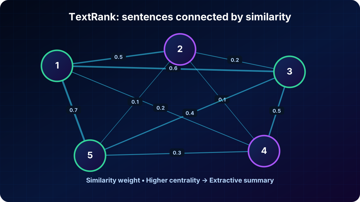
TextRank is an unsupervised graph algorithm. Each sentence can be a node, and edges connect sentences with weights derived from term similarity. Like PageRank, its central idea is that a sentence becomes important when it resembles other important sentences.
Build a graph with sentence nodes and edge weights based on word overlap or cosine similarity between sentence vectors.
Iteratively update each node rank from neighboring scores and weights. The damping factor d is commonly 0.85.
After convergence, select the highest-ranked sentences for the summary.
Connection thickness represents similarity; central nodes are likely to appear in the extractive summary.
In the cloud-computing example, five sentences cover on-demand resources, servers and storage, Azure as Microsoft’s cloud platform, infrastructure cost reduction, and scalability. The ten pairwise weights are 0.5, 0.6, 0.2, 0.7, 0.2, 0.1, 0.1, 0.5, 0.4, and 0.3. Sentences 1, 3, and 5 may receive the highest scores and form a concise summary.
Selecting existing sentences is extractive summarization. Newer semantic models also support abstractive summarization, which writes new language that condenses source themes. TextRank can work at the word level too: terms become nodes, co-occurrence within a window becomes an edge, and top-ranked nodes become key terms.
9. Semantic language models and embeddings
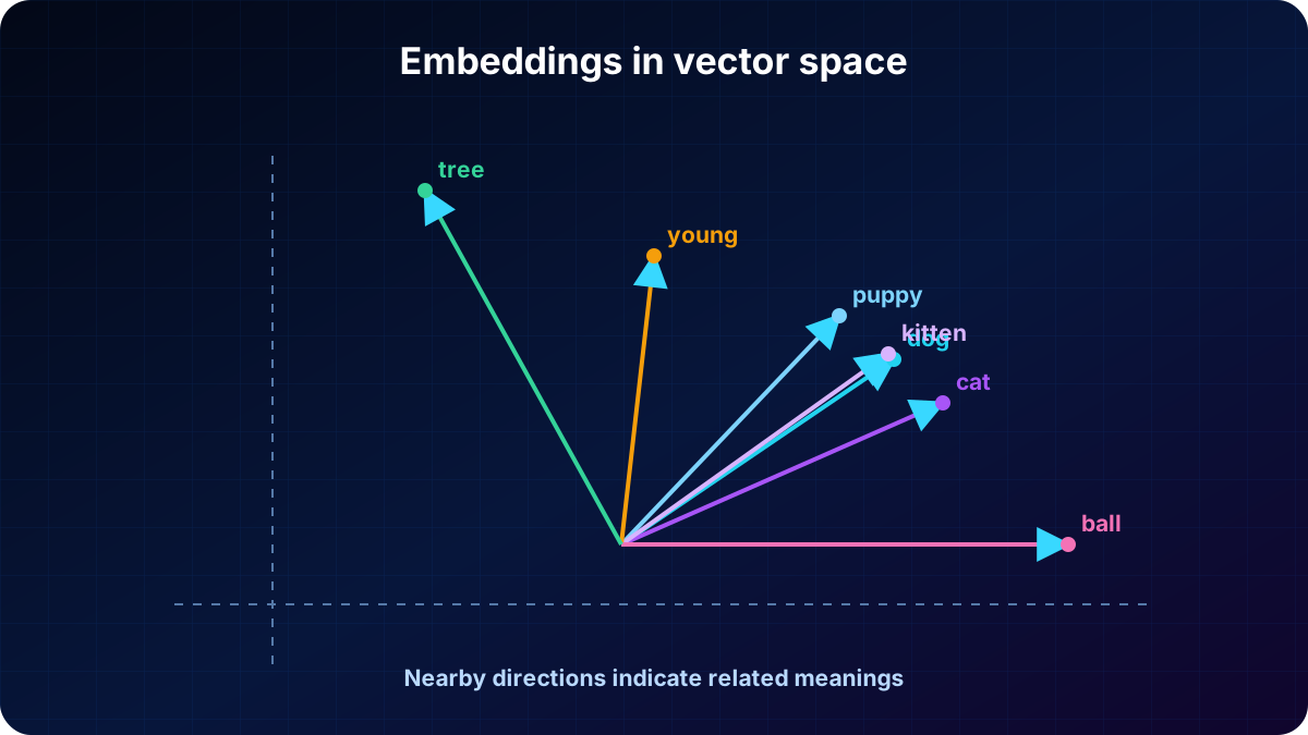
NLP advances produced deep-learning models that represent tokens as dense multidimensional vectors called embeddings. Word2Vec and GloVe popularized this method: during training, dimension values come to reflect semantic characteristics inferred from usage.
Mathematical vector relationships make many analysis tasks more efficient than purely statistical approaches. Attention extended the method by measuring surrounding-token influence and producing contextual embeddings, which underpin modern models such as the GPT family and generative AI.
Teaching example with three-dimensional vectors.
Word
Vector
dog
[0.8, 0.6, 0.1]
puppy
[0.9, 0.7, 0.4]
cat
[0.7, 0.5, 0.2]
kitten
[0.8, 0.6, 0.5]
young
[0.1, 0.1, 0.3]
ball
[0.3, 0.9, 0.1]
tree
[0.2, 0.1, 0.9]
Dog and cat point in nearby directions, as do puppy and kitten, while tree, young, and ball represent different meanings.
10. Cosine similarity and related terms
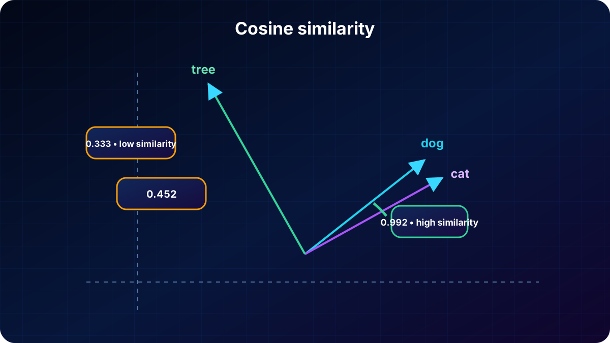
Cosine similarity compares vector orientation. Values near 1 indicate similar directions, while lower values indicate more distant meanings.
cosine_similarity(A,B) = (A · B) / (||A|| × ||B||)
For dog [0.8, 0.6, 0.1] and cat [0.7, 0.5, 0.2], the dot product is 0.88, magnitudes are about 1.005 and 0.883, and similarity is 0.992. Dog and tree produce 0.333; cat and tree, 0.452. Tree is therefore the semantic odd one out.
Dog and cat have almost identical orientations, while tree remains distant from both.
11. Vector arithmetic and analogies
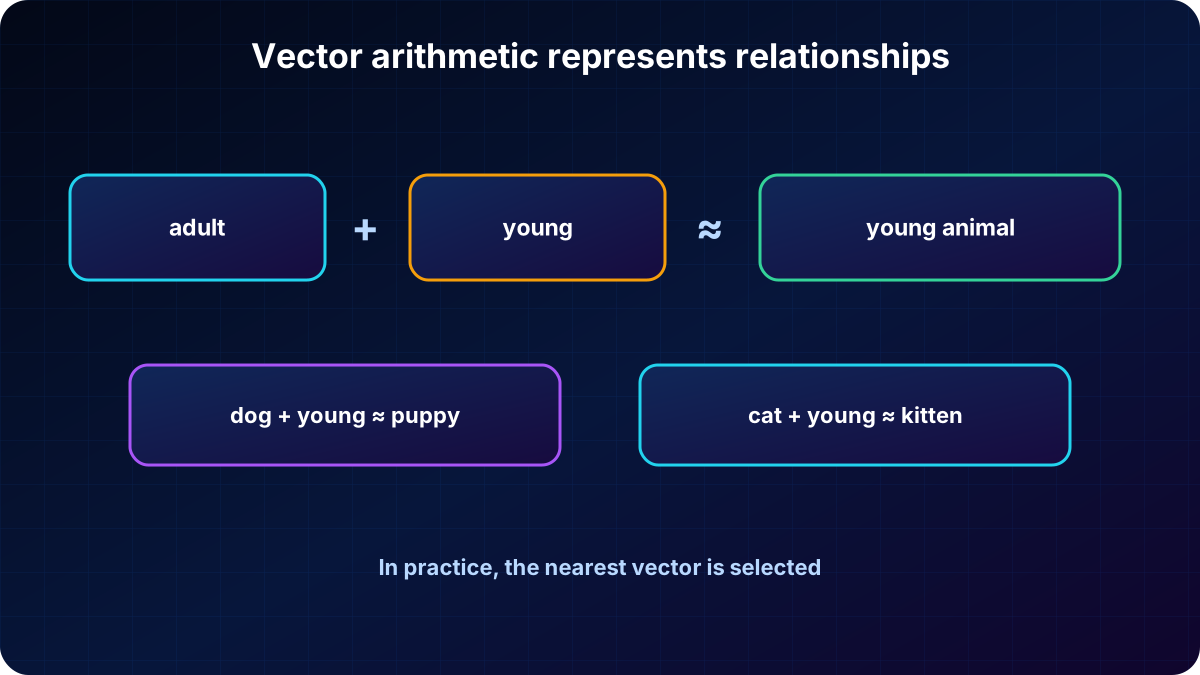
Adding or subtracting embeddings can represent linguistic transformations. With the teaching vectors, dog + young yields [0.9, 0.7, 0.4], or puppy; cat + young yields [0.8, 0.6, 0.5], or kitten.
The relationship also works backward: puppy − young returns dog, and kitten − young returns cat. In production, arithmetic rarely yields an exact match; the system searches for the token vector nearest the result.
The semantic “young” component moves dog and cat vectors toward puppy and kitten.
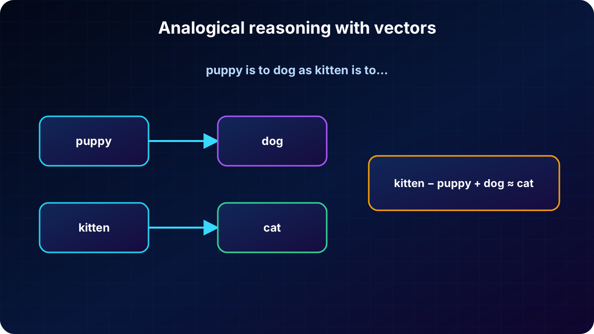
The same idea solves analogies. To complete “puppy is to dog as kitten is to what?”, calculate kitten − puppy + dog. The result [0.7, 0.5, 0.2] matches cat.
Vector operations capture linguistic patterns and enable reasoning over relationships.
12. Text-analysis tasks with semantic models
Using embeddings for text analysis.
Task
Semantic approach
Text summarization
Represents sentences by averaged or pooled embeddings and extracts the most central; generative models can also produce abstractive summaries.
Keyword extraction
Compares word embeddings with the document representation or identifies terms central to all word vectors.
Named entity recognition
Fine-tuned models learn clusters for people, organizations, locations, and other types and use context at inference time.
Text classification
Aggregates embeddings into document vectors for a classifier or compares them directly with class-prototype vectors.
Sentiment analysis
Groups semantically similar documents and separates emotional categories.
13. Exercise and knowledge check
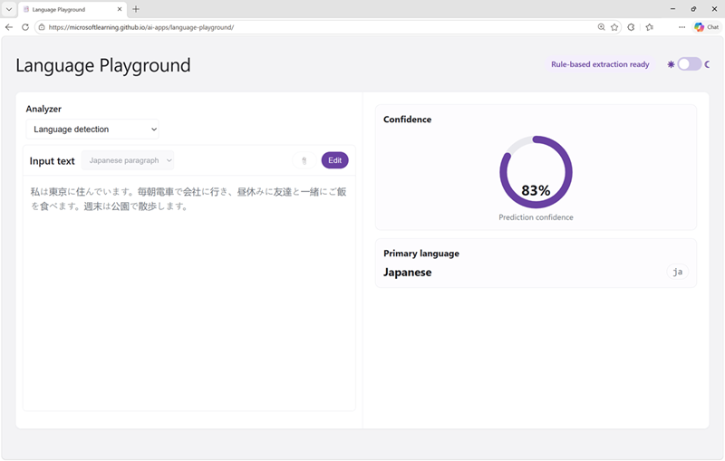
The exercise uses Language Playground to experiment with language tasks and observe how AI analyzes text.
The real interface capture remains a PNG; only conceptual diagrams were redrawn.